VLOOKUP
If you have known information on your spreadsheet, you can use VLOOKUP to search for related information by row. For example, if you want to buy an orange, you can use VLOOKUP to search for the price.
[VLOOKUP for BigQuery]
Syntax
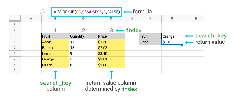
=VLOOKUP(search_key,``range, index, [is_sorted])
Inputs
search_key: The value to search for in the first column of the range.range: The upper and lower values to consider for the search.index: The index of the column with the return value of the range. The index must be a positive integer.is_sorted: Optional input. Choose an option:FALSE= Exact match. This is recommended.TRUE= Approximate match. This is the default ifis_sortedis unspecified. Important: Before you use an approximate match, sort your search key in ascending order. Otherwise, you may likely get a wrong return value. Learn why you may encounter a wrong return value.
Return value
The first matched value from the selected range.
[Technical details:]
Basic VLOOKUP examples:
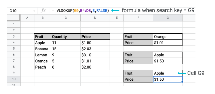
VLOOKUP on different search keys
Use VLOOKUP to find the price of an Orange and Apple.
[Explanation:]
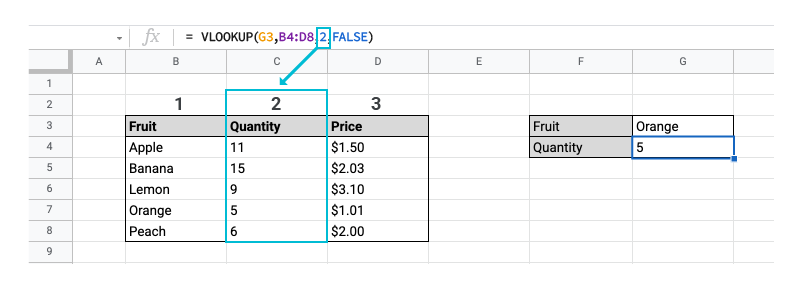
VLOOKUP on different column indexes
Use VLOOKUP to find the quantity of Oranges in the second index column.
[Explanation:]
[VLOOKUP exact match or approximate match]
- Use
VLOOKUPexact match to find an exact ID. - Use
VLOOKUPapproximate match to find the approximate ID.
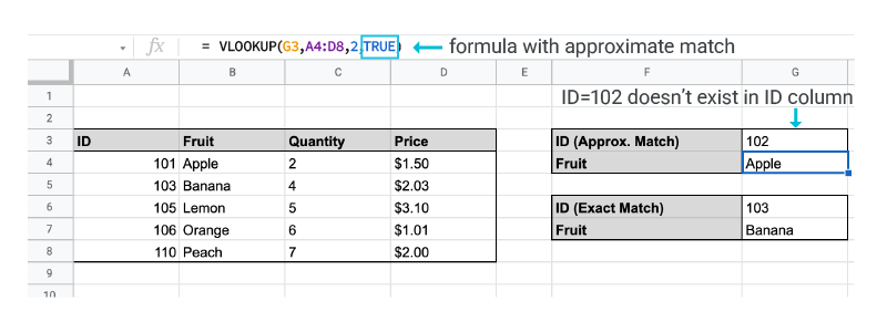
[Explanation:]
Common VLOOKUP applications
[Replace error value from VLOOKUP]
You may want to replace an error value returned by VLOOKUP when your search key doesn’t exist. In this case, if you don’t want #N/A, you can use IFNA functions to replace #N/A. Learn more about IFNA.
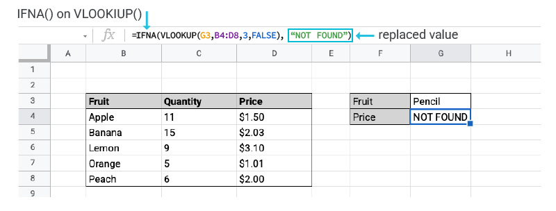
Originally,VLOOKUP returns #N/A because the search key “Pencil” does not exist in the “Fruit” column.IFNA replaces #N/A error with the second input specified in the function. In our case, it’s “NOT FOUND.” | =IFNA(VLOOKUP(G3, B4:D8, 3, FALSE),"NOT FOUND")Return value = “NOT FOUND” |
|---|
Tip: If you want to replace other errors such as #REF!, learn more about IFERROR.
VLOOKUP with multiple criteria
VLOOKUP can’t be directly applied on multiple criteria. Instead, create a new helper column to directly apply VLOOKUP on multiple criteria to combine multiple existing columns.
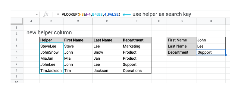
| 1. You can create a Helper column if you use "&" to combine First Name and Last Name. | =C4&D4 and drag it down from B4 to B8 gives you the Helper column. |
|---|---|
| 2. Use cell reference B7, JohnLee, as the search key. | =VLOOKUP(B7, B4:E8, 4, FALSE)Return value = "Support" |
VLOOKUP with wildcard or partial matches
In VLOOKUP, you can also use wildcards or partial matches. You can use these wildcard characters:
- A question mark "?" matches any single character.
- An asterisk "*" matches any sequence of characters.
To use wildcards in VLOOKUP, you must use an exact match: "is_sorted = FALSE".
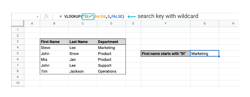
| "St*" is used to match anything that starts with "St" regardless of the number of characters, such as "Steve", "St1", "Stock", or "Steeeeeeve". | =VLOOKUP("St*", B4:D8, 3, FALSE)Return value = "Marketing" |
|---|